Knots and links
A knot is a closed curve in space, and a link consists of several such curves; two are the same if one can be moved to the other without passing through itself. Explore their invariants as you draw and reshape diagrams.
Prime knots and links
In space
This diagram
The knot
Its group
Knot polynomials
To compute the HOMFLYPT polynomial of a diagram, we change the diagram one crossing at a time. First we choose a crossing: in the pictures above it is ringed in red, and clicking another crossing chooses that one. Keeping everything else as it is, we can make it positive (), negative (), or open it along the orientations of the strands (). These are the three pictures, and our diagram is the shaded one. Their polynomials are tied by the skein relation [7, 16]
We solve it for the shaded diagram,
and work out the other two diagrams in the same way [12]. In the end each diagram is reduced to an unlink of components, and in this situation
The other polynomials are values of . Setting and gives the Jones polynomial [9]; setting gives Conway’s polynomial, and from it the Alexander polynomial [3]:
Kauffman’s bracket
The bracket computes the Jones polynomial by opening all the crossings at once. At each crossing we choose A, joining the two corners that the upper strand sweeps when turned anticlockwise, or B, joining the other two; in the picture above, clicking a crossing changes its choice. With the number of loops left, and and the numbers of crossings opened each way, the sum over all choices is
The second and third Reidemeister moves [17] leave unchanged and the first multiplies it by , so correcting for the writhe gives the Jones polynomial [10]:
The span of , its highest power of less its lowest, is at most the crossing number, with equality for an alternating diagram that has no crossing a twist would undo.
The group of the complement
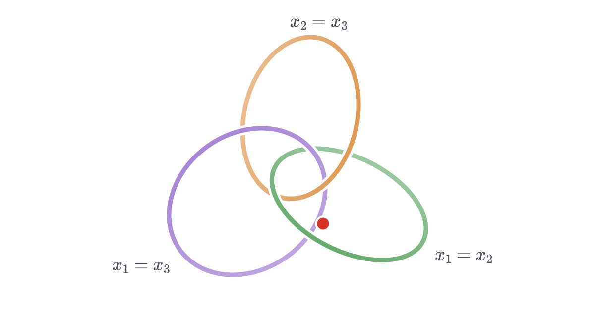
The fundamental group of the complement of the link can be read off a diagram (Wirtinger; see [5]). We cut the diagram wherever it passes under itself; each piece gives a generator, which is the loop once round it. In the picture above the pieces are named, with their orientations marked, and clicking a crossing shows its relation: with the piece on top, and and the pieces that end and begin under it,
One relation follows from the others, and a generator that a relation gives in terms of the others can be left out; what remains is the presentation beside the diagram at the top, where clicking a generator draws all of them as loops.
A knot’s group is only for the unknot [15]. Fox’s free derivatives of the relations, with every generator sent to , give a matrix whose determinant, with a row and a column left out, is up to [1, 5]; the determinant of the link is . At a relation reads
and numbers on the pieces that satisfy it at every crossing are a colouring mod (shown by Colouring): a homomorphism of the group to the dihedral group of order , onto it for a prime if the colouring is not constant. There is one exactly when divides the determinant. Homomorphisms onto other finite groups tell many knots apart [18]; beside the diagram at the top are those onto , and , up to conjugation.
Signature
The signature comes from a surface that the link bounds. We shade the regions of the diagram like a chessboard, as in the picture above, and join the shaded regions by a half-twisted band at each crossing. Let say which way the band at crossing twists. Goeritz’s matrix has a row and a column for each white region but one, with over the crossings that two regions share off the diagonal, and on it what makes each row, with the region left out, sum to zero. Then, with the sign of the crossing,
the sum running over the crossings where the surface cannot be oriented along with the link [8]. The right-handed trefoil has signature .
Genus, braid index and volume
These are least values over all diagrams, or come from the geometry of the complement: a diagram bounds them, and fixes them where the bounds meet.
Opening every crossing along the orientations leaves loops, the Seifert circles. Spanning them by discs, joined by a half-twisted band at each crossing, gives a surface with the link as its edge [20], of genus for a knot. So the genus of a knot satisfies
with equality throughout for an alternating diagram [4, 14].
A closed braid on strands has Seifert circles, and the braid index is the least over all diagrams [24]; the powers of in bound it from below [6, 13]:
The Arf invariant of a knot is when its determinant is mod , and when it is mod [11].
Most links are hyperbolic: their complement has a complete metric of constant curvature , whose volume is an invariant [22]; torus links, sums, split links and satellites are not. To find the volume, we add two points, above and below the diagram, and the complement falls into four tetrahedra at each crossing [21]; squashing an edge from each added point onto the link and simplifying leaves an ideal triangulation. Each tetrahedron is then a shape in the upper half-plane, and Thurston’s equations ask that round every edge the shapes multiply to and that every cusp be complete. Solving them by Newton’s method gives the hyperbolic structure, and
the Bloch–Wigner dilogarithm being the volume of an ideal tetrahedron of shape [22, 23].
Names
Prime knots and links are named as in Rolfsen’s book [19]. Which of a knot and its mirror image is called , and which , follows the Knot Atlas [2].
We name a knot or link by comparing its invariants with those of the table, so the name may be uncertain when the diagram after Tidy has more crossings than the table covers: more than nine for a knot, or seven for a link.